


Getting Started with PyTorch

Jeremy Morgan 
Apr 24, 2023 - 10 min read
Last Update: Apr 24, 2023
AI changed software development. This is how the pros use it.
Written for working developers, Coding with AI goes beyond hype to show how AI fits into real production workflows. Learn how to integrate AI into Python projects, avoid hallucinations, refactor safely, generate tests and docs, and reclaim hours of development time—using techniques tested in real-world projects.
Do you want to learn more about PyTorch? Yeah, me too. I’ve been studying it lately and learning myself. I put together some steps to get started, then asked ChatGPT for a suitable “hello world” type of project for PyTorch. I wanted to create a quick and easy guide to get started, and here we are.
This tutorial will guide you through building a simple PyTorch project that classifies handwritten digits using the MNIST dataset. Our project will create a neural network using PyTorch.
We’ll walk through each step of the process, from setting up a virtual environment and loading the data to training and evaluating the model.
By the end of this tutorial, you’ll know how to create a basic PyTorch project and apply it to real-world problems like digit classification.
In this tutorial, we’ll cover:
- Understanding the basics of PyTorch and its applications.
- Building a simple project using PyTorch
- Learning the essential steps and components involved in a PyTorch project.
So, let’s dive in and start building your first PyTorch project!
Introduction:
So, what is PyTorch, and why should you care? PyTorch is a Python-based library developed by Meta AI (Formerly Facebook AI Research Lab). Pytorch provides tools for creating, training, and deploying deep learning models.
With PyTorch, you can create complex neural networks, harness the power of GPUs, and solve cool problems. It’s used in research, academia, and industry for various applications, including computer vision, natural language processing, and reinforcement learning.
Let’s dive in!
The Process
In our PyTorch project, we will follow three main steps to build and evaluate our digit classification model:
Loading Data: The first step is to load the dataset, which in our case is the MNIST dataset. The torchvision library makes accessing the dataset easy and applying transformations, like converting images to tensors and normalizing pixels. We create separate DataLoaders for training and testing, which handle batching and shuffling data. These DataLoaders will be used to feed data into our neural network during training and evaluation.
Training the Model: The next step is to create a neural network model using the SimpleNet class. We initialize the model, along with the loss function (CrossEntropyLoss) and the optimizer (Adam). Then, we train the model using a training loop that iterates over the training data in batches. In each iteration, we feed the input data through the model, calculate the loss, and update the model’s weights with the optimizer. We repeat this for a set number of epochs to improve the model’s performance.
Evaluating the Model: We test it on a real-world dataset after training the model. We create a separate evaluation function, check_accuracy, that iterates over the test data in batches. Each time we run the model, we compare the predicted and true labels. We calculate the number of correct predictions and the total number of samples to compute the accuracy of our model on the test dataset.
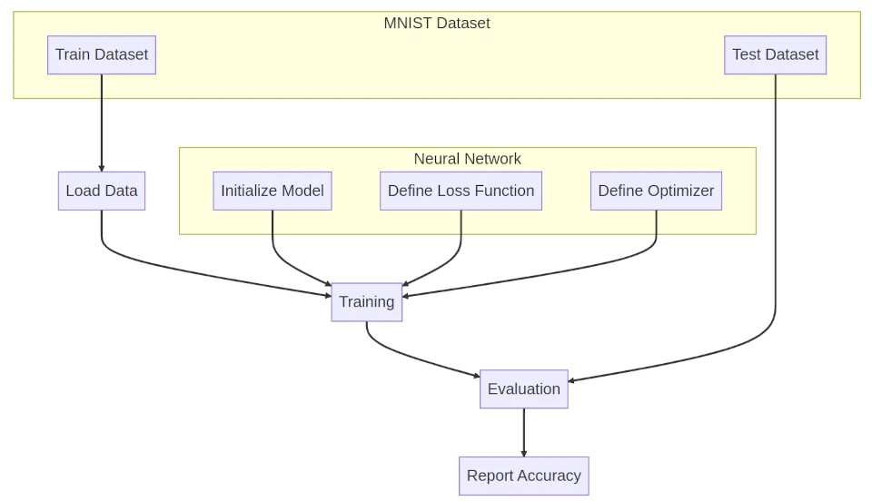
By following these steps, we can create a simple PyTorch project that trains a neural network to classify handwritten digits and evaluates its performance on data.
Step 1: Creating a Python Virtual Environment
You must have Python 3.6 or newer to complete this tutorial.
To create a virtual environment, open your terminal or command prompt, navigate to your project folder, and run
python -m venv pytorchdemo
This command will create a new folder named pytorchdemo in your project directory, containing an isolated Python environment. To activate the virtual environment, run
source pytorchdemo/bin/activate
on macOS/Linux or
pytorchdemo\Scripts\activate
in Windows.
Now you have a virtual environment set up, let’s install Pytorch!
Step 2: Installing PyTorch
Before we can start building our project, we need to have PyTorch installed on our system. To do this, follow the instructions on the official PyTorch installation guide. Many folks use Anaconda, but you can use pip as well. Here is a quick setup that might work for you.
pip install torch torchvision torchaudio
And you should be good to go. If not, consult the documentation. If you have a GPU, PyTorch supports CUDA 11.7 and 11.8.
If you want to install with CUDA 1.8, the command is a little different:
pip install torch torchvision torchaudio --index-url https://download.pytorch.org/whl/cu118
Once you have installed PyTorch, you can verify the install by creating a main.py and adding the following code:
import torch
print(torch.__version__)
And run it:
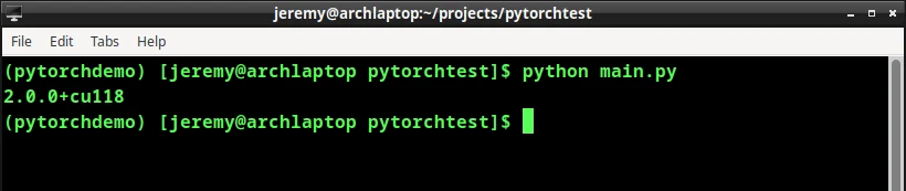
If the output displays the installed PyTorch version, you’re good to go!
Step 3: Importing Libraries
Now that we have PyTorch installed let’s import the necessary libraries to build our project. In this tutorial, we’ll be using the following libraries:
import torch
import torch.nn as nn
import torch.optim as optim
import torchvision.datasets as datasets
import torchvision.transforms as transforms
from torch.utils.data import DataLoader
Step 4: Creating a Neural Network
As mentioned earlier, we will create a simple neural network to classify handwritten digits from the MNIST dataset. First, let’s define our neural network class.
Create a new Python file in your project directory named simplenet.py and add the following code:
import torch
import torch.nn as nn

class SimpleNet(nn.Module):
    def __init__(self, input_size, num_classes):
        super(SimpleNet, self).__init__()
        self.fc1 = nn.Linear(input_size, 50)
        self.fc2 = nn.Linear(50, num_classes)

    def forward(self, x):
        x = torch.relu(self.fc1(x))
        x = self.fc2(x)
        return x
In our SimpleNet class, we define a neural network architecture with two fully connected (linear) layers. These layers transform the input data into a representation that allows the network to learn the relationship between the input (handwritten digit images) and the output (correct digit labels).
Let’s break this down a bit:
fc1 (first fully connected layer) : This layer is the input layer of our neural network. It takes the pixel values of an MNIST image (which is 28x28 pixels) as input and transforms them into a new representation with 50 hidden units (neurons). The input size equals the number of pixels (28x28 = 784). This means each pixel in the image is connected to every hidden unit in the fc1 layer. This layer learns and extracts meaningful features from the input images. This will help the network recognize and classify the handwritten digits.
fc2 (second fully connected layer) : In our neural network, this layer is the output layer. It transforms the output of the first fully connected layer (50 hidden units) into a new representation with 10 output units (neurons). Each output unit corresponds to a digit class (0 to 9). This layer learns the relationship between the features extracted by the fc1 layer and the correct digit labels. The network will use this learned relationship for a given input image to predict the right label.
In our SimpleNet class, we define two fully connected layers that learn to classify handwritten digit images into their correct classes (0 to 9). Beginners like us can use this architecture to see how neural networks work in PyTorch while still solving the MNIST digit classification problem.
to use this class in your app, add the following to main.py:
from simplenet import SimpleNet
Now, we need to load in some data.
Step 5: Loading and Preprocessing the Data
Let’s create a new Python file to train our neural network. Create a file named train.py.
Before training our neural network, we need to load and preprocess the MNIST dataset.
First, let’s define the data transformations, such as normalization:
transform = transforms.Compose([transforms.ToTensor(), transforms.Normalize((0.1307,), (0.30811,))])
Next, let’s download and load the MNIST dataset using torchvision:
train_dataset = datasets.MNIST(root='data/', train=True, transform=transform, download=True)
train_dataset = datasets.MNIST(root='data/', train=True, transform=transform, download=True)
train_loader = DataLoader(train_dataset, batch_size=64, shuffle=True)
Here, we download the training dataset and apply the transform function. We then create a data loader for the training set with a batch size of 64 and shuffling enabled for the training data.
Step 6: Training the Neural Network
Now, it’s time to train our neural network. First, let’s initialize our model, loss function, and optimizer:
input_size = 28 * 28
num_classes = 10
learning_rate = 0.001
num_epochs = 10

model = SimpleNet(input_size, num_classes)
criterion = nn.CrossEntropyLoss()
optimizer = optim.Adam(model.parameters(), lr=learning_rate)
We’ve set the input size, number of classes, learning rate, and number of epochs. We use the cross-entropy loss as our loss function and the Adam optimizer for updating the model parameters.
Next, let’s write the training loop:
for epoch in range(num_epochs):
    for batch_idx, (data, targets) in enumerate(train_loader):
        data = data.reshape(-1, input_size)
        scores = model(data)
        loss = criterion(scores, targets)

        optimizer.zero_grad()
        loss.backward()
        optimizer.step()
In this loop, we iterate over the training data in batches, reshape the input data to match our model’s input size, and compute the scores (model output). We then calculate the loss and perform backpropagation to update the model parameters.
Let’s run it:
python training.py
Note you may hear the fans spinning!
Step 7: Evaluating the Model
Now we need to evaluate our model.
After training, let’s evaluate our model on the test dataset:
at the top of the file, put in our imports:
import torch
import torchvision.datasets as datasets
import torchvision.transforms as transforms
from torch.utils.data import DataLoader
from simplenet import SimpleNet
and we’ll load up the data:
transform = transforms.Compose([transforms.ToTensor(), transforms.Normalize((0.1307,), (0.3081,))])
test_dataset = datasets.MNIST(root='data/', train=False, transform=transform, download=True)
test_loader = DataLoader(test_dataset, batch_size=64, shuffle=False)
Then load in our trained model:
input_size = 28 * 28
num_classes = 10

model = SimpleNet(input_size, num_classes)
model.load_state_dict(torch.load('trained_model.pth'))
Next, we need to create our check_accuracy function:
def check_accuracy(loader, model):
    num_correct = 0
    num_samples = 0
    model.eval()

    with torch.no_grad():
        for x, y in loader:
            x = x.reshape(-1, input_size)
            scores = model(x)
            _, predictions = torch.max(scores, 1)
            num_correct += (predictions == y).sum()
            num_samples += predictions.size(0)

    model.train()
    return num_correct / num_samples
and finally, we’ll display our results:
print(f"Accuracy on test dataset: {check_accuracy(test_loader, model):.2f}")
This function calculates the accuracy of our model on the given data loader (in this case, the test dataset). We set the model to evaluation mode and disable gradient computation to improve performance during testing. Finally, we print the accuracy of our model on the test dataset.
Let’s run it!
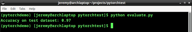
Very nice!
This is a metric used to evaluate the performance of a machine learning model. In our case, it represents how well our trained neural network can correctly classify handwritten digits from the MNIST dataset that it has not seen before.
The test dataset is a separate portion of the data, not used during training, ensuring that the model’s performance is measured on unseen examples. So “Accuracy on test dataset” is an estimate of how well our trained neural network generalizes to new, unseen data. It helps us understand the effectiveness of our model in solving the digit classification problem.
But this is just a number. Let’s show the model in action. To do this, we’ll plot out some visuals.
Step 8: Using the Model
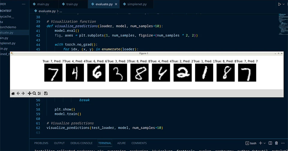
To demonstrate the model in action, we will add a section to the evaluate.py file showing some sample images from the test dataset, their true labels, and the model’s predictions.
First, we’ll install matplotlib (one of my favorites!)
pip install matplotlib
Then modify the evaluate.py file like this:
add this to the top:
import matplotlib.pyplot as plt
then add this function and its call:
# Visualization function
def visualize_predictions(loader, model, num_samples=10):
    model.eval()
    fig, axes = plt.subplots(1, num_samples, figsize=(num_samples * 2, 2))

    with torch.no_grad():
        for idx, (x, y) in enumerate(loader):
            x = x.reshape(-1, input_size)
            scores = model(x)
            _, predictions = torch.max(scores, 1)

            # Plot sample image, true label, and predicted label
            axes[idx].imshow(x[idx].reshape(28, 28).numpy(), cmap='gray')
            axes[idx].set_title(f"True: {y[idx].item()}, Pred: {predictions[idx].item()}")
            axes[idx].axis("off")

            if idx == num_samples - 1:
                break

    plt.show()
    model.train()

# Visualize predictions
visualize_predictions(test_loader, model, num_samples=10)
And run it again:
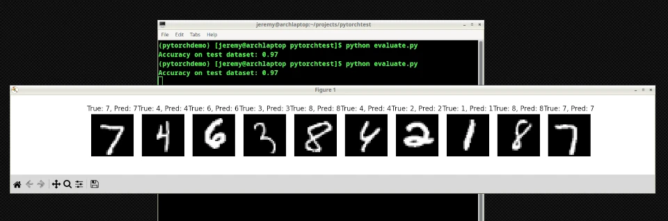
Awesome right? Here we can see a visual representation of our model in action.
Soon on this blog, we’ll introduce our own data into the mix and try it out.
Conclusion:
Congratulations, you’ve just built your first PyTorch project! In this tutorial, you learned:
- The basics of PyTorch and its applications.
- How to build a simple project using PyTorch to demonstrate its capabilities.
- The essential steps and components involved in a PyTorch project include creating a neural network, loading and preprocessing data, training, and evaluation.
Now you know how to build a simple PyTorch project! With PyTorch, you can tackle deep learning problems and create state-of-the-art models. I am learning more about this every day, and you can too!
Bookmark this blog and come back for more cool Pytorch projects.

Skip the hype. The newsletter that keeps you in the know.
AI news curated for engineers. The AI New Hotness Newsletter is what you need.
Zero fluff. Just the research, tools, and infra updates that actually affect your production stack.
Stay up to date on AI for developers - Subscribe on LinkedIn